Model Diagnostics & Spatial Autocorrelation

Week 7: CPLN 5920-MUSA 5080

Dr. Allison Lassiter

2026-03-02

Homework Feedback & Tips

Before We Start: A Quick Note on Lab 2 Submissions

Many of you have messy output in your rendered HTML files from tigris and tidycensus functions.

Example of what we’re seeing:

Retrieving data for the year 2022
  |======================================================================| 100%
  |======================================================================| 100%
Downloading: 4.3 MB     
Downloading: 3.7 MB

This clutters your professional report!

The Problem: Progress Bars in Rendered Output

What’s happening:

When you use tigris or tidycensus functions, they show download progress by default.

In your console (good!):

tracts <- get_acs(
  geography = "tract",
  variables = "B01003_001",
  state = "PA",
  geometry = TRUE
)

Shows:

Getting data from the 2018-2022 5-year ACS
  |======| 100%

This is helpful when coding!

In your rendered HTML (bad!):

All those progress messages appear as ugly text in your final document.

This looks unprofessional and makes your work harder to read.

Solution: Suppress progress messages in your code chunks

The Solution: Add `progress = FALSE`

Two ways to fix this:

Option 1: In each function call

# Add progress = FALSE to EVERY tigris/tidycensus call
tracts <- get_acs(
  geography = "tract",
  variables = "B01003_001",
  state = "PA",
  geometry = TRUE,
  progress = FALSE  # <-- Add this!
)

roads <- roads(state = "PA", 
               county = "Philadelphia",
               progress = FALSE)  # <-- Add this!

Option 2: Set globally at top of document (Recommended!)

# Add this near the top of your .qmd after loading libraries
options(tigris_use_cache = TRUE)
options(tigris_progress = FALSE)  # Suppress tigris progress bars

Suggestion: Re-Render

Please go back to your homework and:

Open your .qmd file
Add progress = FALSE to all get_acs(), get_decennial(), and tigris function calls
- OR add the global options at the top of your document
Re-render your document (Click “Render” button)
Check that the HTML output is clean

Today’s Plan

Agenda Overview

Part 1: Review & Connect

Where we’ve been and where we’re going
The regression workflow so far

Part 2: More Model Quality Evaluation

Train/test splits vs. cross-validation review
Spatial patterns in errors
Introduction to spatial autocorrelation

Part 3: Moran’s I as a Diagnostic

Understanding spatial clustering
Calculating and interpreting Moran’s I
Local vs. global measures

Part 4: Midterm Work Session

Part 1: Where We Are

The Journey So Far

Weeks 1-4: Data foundations

Census data, tidycensus, spatial data basics
Visualization and exploratory analysis
Data cleaning

Week 5: Linear regression fundamentals

Y = f(X) + ε framework
Train/test splits, cross-validation
Checking assumptions

Week 6: Expanding the toolkit

Categorical variables, polynomials, and interactions
Spatial features (buffers, kNN, distance)
Neighborhood fixed effects

Last Week’s Key Innovation

You learned to create spatial features:

# Buffer aggregation
crimes_500ft <- count_features_in_buffer(houses, crimes, 500)

# k-Nearest Neighbors
crime_nn3 <- average_distance_to_knn(houses, crimes, k=3)

# Dummy variable and Fixed effects
lm(SalePrice ~ ... + as.factor(neighborhood))

Today’s Question:

How do we know if our model has spatial structure in its errors?

If errors are spatially clustered, we’re missing something important!

The Regression Workflow (Updated)

Building the model:

Visualize relationships
Engineer features
Fit the model
Evaluate performance (RMSE, R²)
Check assumptions

NEW: Spatial diagnostics:

Are errors random or clustered?
Do we predict better in some areas?
Is there remaining spatial structure?

Why This Matters

If errors cluster spatially, it suggests:

Missing spatial variables
Misspecified relationships
Non-stationarity (relationships vary across space)

Part 2: Understanding Spatial Patterns in Errors

What Are Model Errors?

For \[Y_i = f(X_i) + \epsilon_i\]

Prediction error for observation i:

\[e_i = \hat{y}_i - y_i\]

Where:

$\hat{y}_i$ = predicted value
$y_i$ = actual value

In our house price context:

# Load packages and data
library(sf)
library(here)
library(tidyverse)

# Load Boston housing data
boston <- read_csv(here("data/boston.csv"))

# Simple model: Predict price from living area
baseline_model <- lm(SalePrice ~ LivingArea, data = boston)
summary(baseline_model)


Call:
lm(formula = SalePrice ~ LivingArea, data = boston)

Residuals:
    Min      1Q  Median      3Q     Max 
-855962 -219491  -68291   55248 9296561 

Coefficients:
             Estimate Std. Error t value Pr(>|t|)    
(Intercept) 157968.32   35855.59   4.406 1.13e-05 ***
LivingArea     216.54      14.47  14.969  < 2e-16 ***
---
Signif. codes:  0 '***' 0.001 '**' 0.01 '*' 0.05 '.' 0.1 ' ' 1

Residual standard error: 563800 on 1483 degrees of freedom
Multiple R-squared:  0.1313,    Adjusted R-squared:  0.1307 
F-statistic: 224.1 on 1 and 1483 DF,  p-value: < 2.2e-16

boston_test <- boston %>%
  mutate(
    predicted = predict(baseline_model, boston),
    error = predicted - SalePrice,
    abs_error = abs(error),
    pct_error = abs(error) / SalePrice
  )

Good Errors vs. Bad Errors

** Random errors (good)**

No systematic pattern
Scattered across space
Prediction equally good everywhere
Model captures key relationships

** Clustered errors (bad)**

Spatial pattern visible
Under/over-predict in areas
Model misses something about location
Need more spatial features!

How do we test this?

Look for spatial autocorrelation in the errors

Tobler’s First Law (Revisited)

The First Law of Geography

“Everything is related to everything else, but near things are more related than distant things.”

— Waldo Tobler (1970)

Applied to house prices:

Nearby houses have similar prices
Nearby neighborhoods have similar characteristics
Crime in one block affects adjacent blocks

Applied to model errors:

If nearby houses have similar, spatial errors…
…our model is missing a spatial pattern!
Need to add more spatial features or fixed effects

Visualizing Error Patterns

Map your errors to see patterns:

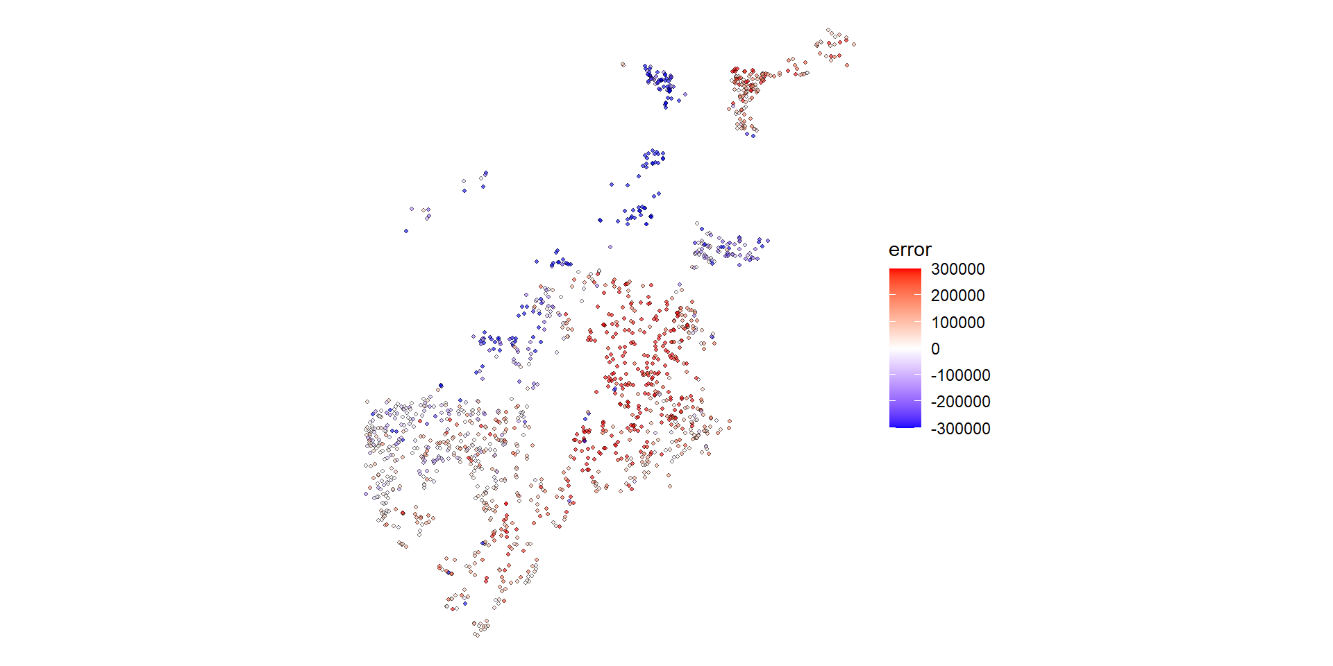
What to look for:

Blue clusters (we under-predict)
Red clusters (we over-predict)
Random scatter (good!)

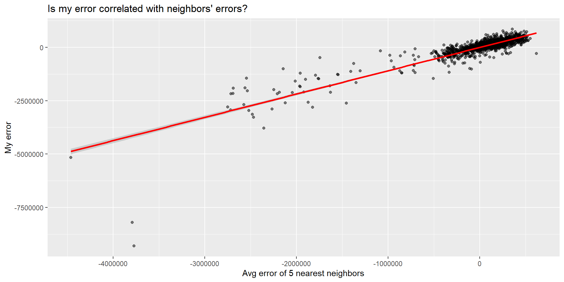
Scatter Plot: Spatial Lag of Errors

Create the spatial lag:

library(spdep)

# Define neighbors (5 nearest)
coords <- st_coordinates(boston_test)
neighbors <- knn2nb(knearneigh(coords, k=5))
weights <- nb2listw(neighbors, style="W") #"W" style gives neighbor average, most useful to us

# Calculate spatial lag of errors
boston_test$error_lag <- lag.listw(weights, boston_test$error)

Then plot:

Part 3: Moran’s I

What is Moran’s I?

Moran’s I measures spatial autocorrelation

“When I’m above/below average, are my neighbors also above/below average?”

Range: -1 to +1

+1 = Perfect positive correlation (clustering)
0 = Random spatial pattern
-1 = Perfect negative correlation (dispersion)

Formula (look’s scary, but its so intuitive!):

\[I = \frac{n \sum_i \sum_j w_{ij}(x_i - \bar{x})(x_j - \bar{x})}{\sum_i \sum_j w_{ij} \sum_i (x_i - \bar{x})^2}\]

Where $w_{ij}$ = spatial weight between locations i and j,
$n$ is the number of observations

Worked Example: Understanding the Formula

5 houses, predicting sale prices:

House	Actual Price	Predicted Price	Error
A	$500k	$400k	+$100k
B	$480k	$400k	+$80k
C	$420k	$400k	+$20k
D	$350k	$400k	-$50k
E	$330k	$400k	-$70k

Mean error = +$16k

The question: Are errors for nearby houses similar to each other?

Step 1: Calculate Deviations from Mean

Subtract the mean error from each house’s error:

House	Error	Mean Error	Deviation from Mean
A	+$100k	+$16k	+$84k
B	+$80k	+$16k	+$64k
C	+$20k	+$16k	+$4k
D	-$50k	+$16k	-$66k
E	-$70k	+$16k	-$86k

Positive deviation = we over-predicted (actual > predicted)
Negative deviation = we under-predicted (actual < predicted)

Step 2: Multiply Neighbor Deviations

For each neighbor pair, multiply their deviations:

Neighbor Pairs:

A-B: $(+84k) \times (+64k) = +5,376$
B-C: $(+64k) \times (+4k) = +256$
C-D: $(+4k) \times (-66k) = -264$
D-E: $(-66k) \times (-86k) = +5,676$

Sum of products = 11,044

What does this mean?

Positive products = similar neighbors - A-B: both over-predicted (both positive) - D-E: both under-predicted (both negative)

Negative product = dissimilar neighbors
- C-D: one over, one under

Result:

Lots of positive products → High Moran’s I (clustering)
Products near zero → Low Moran’s I (random)
Negative products → Negative Moran’s I (rare with errors)

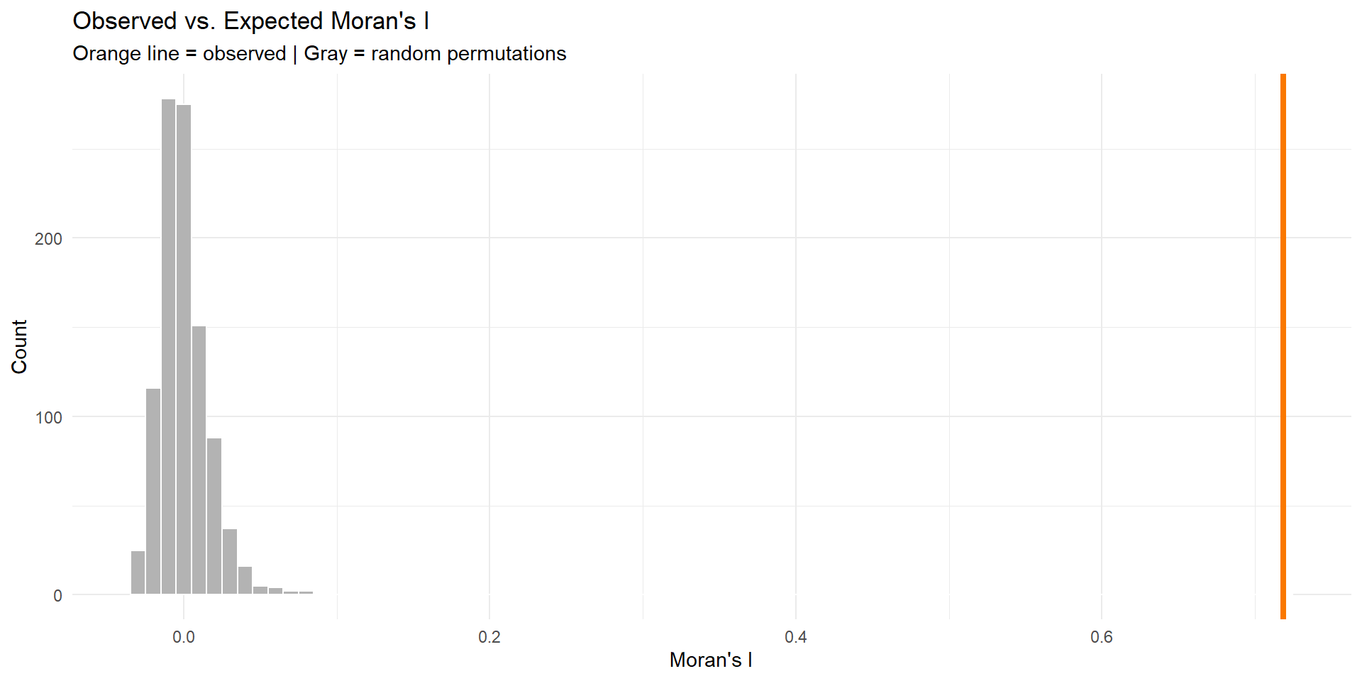
Computing Moran’s I

Calculate Moran’s I for your errors:

# Test for spatial autocorrelation in errors
moran_test <- moran.mc(
  boston_test$error,        # Your errors
  weights,                  # Spatial weights matrix
  nsim = 999                # Number of permutations
)

# View results
moran_test$statistic         # Moran's I value

statistic 
0.7186593

moran_test$p.value          # Is it significant?

[1] 0.001

Interpretation:

I > 0 and p < 0.05 → Significant clustering
I ≈ 0 → Random pattern (good!)
I < 0 → Dispersion (rare with errors)

Visualizing Significance

Compare observed I to random permutations:

What Moran’s I Tells You

Decision Framework

If Moran’s I is high (errors clustered):

Add more spatial features
- Try different buffer sizes
- Include more amenities/disamenities
- Create neighborhood-specific variables
Try spatial fixed effects
- Neighborhood dummies
- Grid cell dummies
Consider spatial regression models
- Spatial lag model
- Spatial error model
- (Advanced topic, not covered today)

If Moran’s I ≈ 0 (random errors):

✅ Your model adequately captures spatial relationships!

Defining “Neighbors”

Different ways to define spatial relationships:

Contiguity

Polygons that share a border
Queen vs. Rook

Distance

All within X meters
Fixed threshold

k-Nearest

Closest k points
Adaptive distance

For point data (houses), use k-nearest neighbors

# Create 5-nearest neighbors
coords <- st_coordinates(boston_test)
nb <- knn2nb(knearneigh(coords, k=5))
weights <- nb2listw(nb, style="W")

New term: Spatial Lag

Spatial lag = average value of neighbors

Example: 5 houses

House	Sale Price	2 Nearest	Spatial Lag
A	$200k	B, C	$275k
B	$250k	A, C	$250k
C	$300k	B, D	$275k
D	$350k	C, E	$350k
E	$400k	D	$350k

In R:

boston$price_lag <- lag.listw(weights, boston$SalePrice)

“What About Spatial Lag/Error Models?”

“In my spatial statistics class, I learned about spatial lag and spatial error models for dealing with spatial autocorrelation. Why aren’t we using those here?”

Spatial Econometrics Models

(Spatial Statistics Class)

Spatial Lag Model: $Y_i = \rho WY + \beta X_i + \varepsilon$

Spatial Error Model: $Y_i = \beta X_i + \lambda W\varepsilon + \xi$

Purpose:

Causal inference with spatial spillovers
Understanding neighbor effects
Correct standard errors for hypothesis testing
Cross-sectional analysis

When to use: Academic research on spillover effects, peer influence, regional economics

Predictive Spatial Features

(This Class)

Our Approach: \[Y_i = \beta_0 + \beta_1 X_i + \beta_2(\text{crimes}_{500ft}) + \beta_3(\text{dist}_{downtown}) + \varepsilon_i\]

Purpose:

Out-of-sample prediction
Forecasting new observations
Applied machine learning
Generalization to new areas

When to use: Real estate prediction, housing market forecasting, policy planning

Why Not Spatial Lag Models for Prediction?

1. Simultaneity Problem

Including $WY$ (neighbor prices) creates circular logic
My price affects neighbors → neighbors affect me

2. Prediction Paradox

Need neighbors’ prices to predict my price
But for new developments or future periods, those prices don’t exist yet
Can’t generalize to truly new areas

3. Data Leakage in CV

Geographic CV holds out spatial regions
Spatial lag “leaks” information from test set
Artificially good performance that won’t hold

Our Solution: Spatial Features of X (Not Y)

Instead of modeling dependence in Y (prices), model proximity in X (predictors)

❌ Spatial Lag	✅ Our Approach
“Near expensive houses”	“Near low crime areas”
Uses neighbor prices	Uses neighbor characteristics
Circular logic	Causal mechanism
Can’t predict new areas	Generalizes well

If Moran’s I shows clustered errors:

✅ Add more spatial features (different buffers, more amenities)
✅ Try neighborhood fixed effects
✅ Use spatial cross-validation

❌ Don’t add spatial lag of Y for prediction purposes

The Bottom Line

Both approaches are valid for different goals! Match method to purpose: inference → spatial lag/error models; prediction → spatial features.

Summary & Next Steps

Key Takeaways

Spatial autocorrelation in errors indicates model misspecification

Moran’s I is a diagnostic tool:

Global I: overall clustering
Maps of residuals give clues to what you might be missing

Iterative improvement:

Diagnose → Engineer features → Re-test → Repeat
Document what you try!

Resources

Spatial autocorrelation: - https://mgimond.github.io/Spatial/spatial-autocorrelation.html

spdep package: - https://r-spatial.github.io/spdep/

Model Diagnostics & Spatial Autocorrelation

Homework Feedback & Tips

Before We Start: A Quick Note on Lab 2 Submissions

The Problem: Progress Bars in Rendered Output

In your console (good!):

In your rendered HTML (bad!):

The Solution: Add progress = FALSE

Option 1: In each function call

Option 2: Set globally at top of document (Recommended!)

Suggestion: Re-Render

Today’s Plan

Agenda Overview

Part 1: Where We Are

The Journey So Far

Last Week’s Key Innovation

The Regression Workflow (Updated)

Part 2: Understanding Spatial Patterns in Errors

What Are Model Errors?

Good Errors vs. Bad Errors

Tobler’s First Law (Revisited)

Visualizing Error Patterns

Scatter Plot: Spatial Lag of Errors

Part 3: Moran’s I

What is Moran’s I?

Worked Example: Understanding the Formula

Step 1: Calculate Deviations from Mean

Step 2: Multiply Neighbor Deviations

Computing Moran’s I

Visualizing Significance

What Moran’s I Tells You

Defining “Neighbors”

New term: Spatial Lag

“What About Spatial Lag/Error Models?”

Spatial Econometrics Models

Predictive Spatial Features

Why Not Spatial Lag Models for Prediction?

Our Solution: Spatial Features of X (Not Y)

Summary & Next Steps

Key Takeaways

Resources

The Solution: Add `progress = FALSE`